Training a 4B model to produce 81% faster query plans than Postgres How good are query optimizers, really? Leis et al. asked this exact question in 2015. Then, they asked it again 10 years later. Des
By Coderz Club · 2026-09-17 · Tags: ai
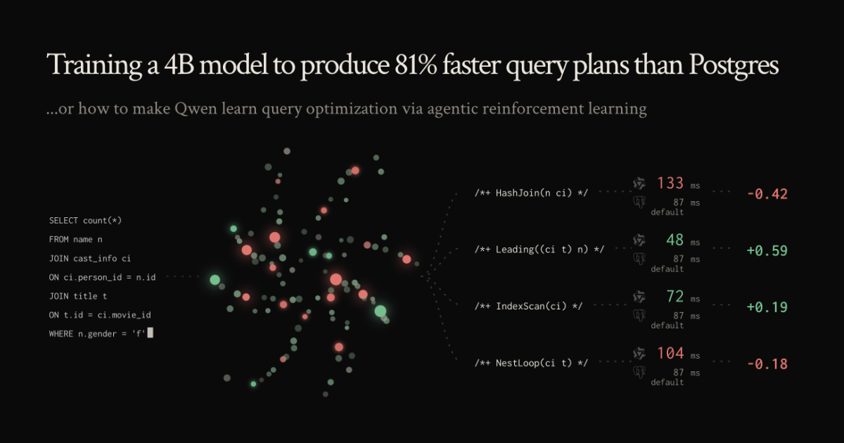
Training a 4B model to produce 81% faster query plans than Postgres
How good are query optimizers, really? Leis et al. asked this exact question in 2015. Then, they asked it again 10 years later. Despite an enormous body of research spanning a decade since their original exploration, they found that query optimizers continue to leave much to be desired. I was surprised when I first learned about this. A Postgres database should know everything about the stuff that lives in its tables, no? How hard can it be? As it turns out: enormously hard. In fact, one particular task a query optimizer needs to do, join ordering, is known to be NP-hard. So query optimizers are hard. What’s not as hard is verifying whether a query plan an optimizer picks is good or not. Put simply, a good query optimizer produces plans that run fast, and a bad one produces slow plans. Language models are particularly good at learning how to do tasks with easily verifiable outputs. Because there’s a single axis to optimize for—execution time of a query—the problem beautifully reduces to reinforcing the behaviors that guide a model to produce faster query plans. What follows is a breakdown of an experiment I ran to explore the question: can a small, open-weights model be post-trained via supervised fine-tuning (SFT) and agentic reinforcement learning (RL) to produce Postgres query plans that beat Postgres’s default plans? The answer to our question is a resounding yes. Highlights include: Attaining a 44.7% latency reduction across 113 join-heavy queries from a 4B model initially unable to produce a query plan for 99 of them Constructing a Postgres measurement rig that minimizes Linux page cache contention noise across concurrent containers Designing a custom GRPO variant for scoring RL rollouts in an inherently noisy environment Splitting RL across two machines: vLLM and the trainer on a rented 2x H100 node and four Postgres containers running on my desk Running off-policy distillation across half a thousand GPT-6 Astra agent trajectories Let’s start from the beginning. Inside a query optimizer Consider the following slice of the IMDb dataset: -- An IMDb title (movie, series, episode, etc.) [~1M rows] title ( id integer PRIMARY KEY, title text, production_year integer, kind_id integer -- FK -> kind_type ) -- Movie <> company junction table [~2M rows] movie_companies ( id integer PRIMARY KEY, movie_id integer, -- FK -> title.id company_id integer, -- FK -> company_name.id company_type_id integer, -- FK -> company_type.id note text ) -- A company s name, origin, etc. [~100k rows] company_name ( id integer PRIMARY KEY, name text, country_code text -- [us] , [jp] , ... ) -- Lookup table of company roles for a title [4 rows] company_type ( id integer PRIMARY KEY, kind text -- production companies , distributors , ... ) -- Lookup table for what a title _is_ [7 rows] kind_type ( id integer PRIMARY KEY, kind text -- movie , tv series , episode , ... ) Let’s say I’m trying to answer the question: “Which Japanese companies put out the most titles in the 2000s?” We might write the following query: SELECT cn.name, COUNT(*) AS titles FROM title AS t, movie_companies AS mc, company_name AS cn WHERE t.id = mc.movie_id AND mc.company_id = cn.id AND cn.country_code = [jp] AND t.production_year BETWEEN 2000 AND 2009 GROUP BY cn.name ORDER BY titles DESC LIMIT 10; Running this query outputs 10 Japanese companies with the number of titles they were associated with between 2000 and 2009, sorted from highest to lowest. But how did Postgres get these results? The path Postgres took to get this data for us is not a foregone conclusion, and it has everything to do with what we call selective predicates (i.e. the filtering conditions in a WHERE clause). To illustrate this, let’s imagine our same query without the Japanese company filter or the date range filter: SELECT cn.name, COUNT(*) AS titles FROM title AS t, movie_companies AS mc, company_name AS cn WHERE t.id = mc.movie_id AND mc.company_id = cn.id GROUP BY cn.name ORDER BY titles DESC LIMIT 10; mc can only join with cn via mc.company_id = cn.id, and t can only join with mc via t.id = mc.movie_id. These constraints produce two There are technically eight join trees if we take commutativity into account. In this case, we don’t because it doesn’t affect the size of the relations resulting from the joins. valid join trees: The two join trees for our query. The lower join runs first; the result is an input into the root join. The cardinality of a table or query result is the number of rows it contains. Assume the relevant tables have the following cardinalities: cn=100kcn = 100\text{k}cn=100k mc=2mmc = 2\text{m}mc=2m t=1mt = 1\text{m}t=1m Taking into account our joins, we get the following cardinalities: (cn⋈mc)=2m, then ⋈t=2m(cn \bowtie mc) = 2\text{m}, \text{ then } \bowtie t = 2\text{m}(cn⋈mc)=2m, then ⋈t=2m (t⋈mc)=2m, then ⋈cn=2m(t \bowtie mc) = 2\text{m}, \text{ then } \bowtie cn = 2\text{m}(t⋈mc)=2m, then ⋈c
How good are query optimizers, really? Leis et al. asked this exact question in 2015. Then, they asked it again 10 years later. Despite an enormous body of research spanning a decade since their original exploration, they found that query optimizers continue to leave much to be desired. I was surprised when I first learned about this. A Postgres database should know everything about the stuff that lives in its tables, no? How hard can it be? As it turns out: enormously hard. In fact, one particular task a query optimizer needs to do, join ordering, is known to be NP-hard. So query optimizers are hard. What’s not as hard is verifying whether a query plan an optimizer picks is good or not. Put simply, a good query optimizer produces plans that run fast, and a bad one produces slow plans. Language models are particularly good at learning how to do tasks with easily verifiable outputs. Because there’s a single axis to optimize for—execution time of a query—the problem beautifully reduces to reinforcing the behaviors that guide a model to produce faster query plans. What follows is a breakdown of an experiment I ran to explore the question: can a small, open-weights model be post-trained via supervised fine-tuning (SFT) and agentic reinforcement learning (RL) to produce Postgres query plans that beat Postgres’s default plans? The answer to our question is a resounding yes. Highlights include: Attaining a 44.7% latency reduction across 113 join-heavy queries from a 4B model initially unable to produce a query plan for 99 of them Constructing a Postgres measurement rig that minimizes Linux page cache contention noise across concurrent containers Designing a custom GRPO variant for scoring RL rollouts in an inherently noisy environment Splitting RL across two machines: vLLM and the trainer on a rented 2x H100 node and four Postgres containers running on my desk Running off-policy distillation across half a thousand GPT-6 Astra agent trajectories Let’s start from the beginning. Inside a query optimizer Consider the following slice of the IMDb dataset: -- An IMDb title (movie, series, episode, etc.) [~1M rows] title ( id integer PRIMARY KEY, title text, production_year integer, kind_id integer -- FK -> kind_type ) -- Movie <> company junction table [~2M rows] movie_companies ( id integer PRIMARY KEY, movie_id integer, -- FK -> title.id company_id integer, -- FK -> company_name.id company_type_id integer, -- FK -> company_type.id note text ) -- A company s name, origin, etc. [~100k rows] company_name ( id integer PRIMARY KEY, name text, country_code text -- [us] , [jp] , ... ) -- Lookup table of company roles for a title [4 rows] company_type ( id integer PRIMARY KEY, kind text -- production companies , distributors , ... ) -- Lookup table for what a title _is_ [7 rows] kind_type ( id integer PRIMARY KEY, kind text -- movie , tv series , episode , ... ) Let’s say I’m trying to answer the question: “Which Japanese companies put out the most titles in the 2000s?” We might write the following query: SELECT cn.name, COUNT(*) AS titles FROM title AS t, movie_companies AS mc, company_name AS cn WHERE t.id = mc.movie_id AND mc.company_id = cn.id AND cn.country_code = [jp] AND t.production_year BETWEEN 2000 AND 2009 GROUP BY cn.name ORDER BY titles DESC LIMIT 10; Running this query outputs 10 Japanese companies with the number of titles they were associated with between 2000 and 2009, sorted from highest to lowest. But how did Postgres get these results? The path Postgres took to get this data for us is not a foregone conclusion, and it has everything to do with what we call selective predicates (i.e. the filtering conditions in a WHERE clause). To illustrate this, let’s imagine our same query without the Japanese company filter or the date range filter: SELECT cn.name, COUNT(*) AS titles FROM title AS t, movie_companies AS mc, company_name AS cn WHERE t.id = mc.movie_id AND mc.company_id = cn.id GROUP BY cn.name ORDER BY titles DESC LIMIT 10; mc can only join with cn via mc.company_id = cn.id, and t can only join with mc via t.id = mc.movie_id. These constraints produce two There are technically eight join trees if we take commutativity into account. In this case, we don’t because it doesn’t affect the size of the relations resulting from the joins. valid join trees: The two join trees for our query. The lower join runs first; the result is an input into the root join. The cardinality of a table or query result is the number of rows it contains. Assume the relevant tables have the following cardinalities: cn=100kcn = 100\text{k}cn=100k mc=2mmc = 2\text{m}mc=2m t=1mt = 1\text{m}t=1m Taking into account our joins, we get the following cardinalities: (cn⋈mc)=2m, then ⋈t=2m(cn \bowtie mc) = 2\text{m}, \text{ then } \bowtie t = 2\text{m}(cn⋈mc)=2m, then ⋈t=2m (t⋈mc)=2m, then ⋈cn=2m(t \bowtie mc) = 2\text{m}, \text{ then } \bowtie cn = 2\text{m}(t⋈mc)=2m, then ⋈c